Benchmark of the semi-analytical model in Geoloop with the numerical model, for a triple U-tube
Note
The example is located in the following
working directory: geoloop/examples/benchmark/FINVOL_benchmark
This example demonstrates the benchmark of the semi-analytical model in Geoloop with the numerical model (Cazorla-Marin, 2019; 2021; Cazorla-Marin et al., 2020) in Geoloop.
A triple U-tube is simulated down to 500 meters, for a synthetic subsurface thermal conductivity model with a mix of 70% sand and 30% clay. The inlet temperature and flowrate are fixed for a simulation period of about 1 month with time steps of 1 hour. The simulations include 15 depth-segments, which is around the maximum nr. of segments for the numerical model in the current set-up with a triple U-tube. In radial direction, 20 meters distance is simulated in 20 cells.
It is important to set a sufficient radial distance in the numerical simulations, to avoid an effect of the no-flow boundary condition.
The BHE design and parameters of the benchmark simulations are provided in the table below and Fig. 1.
| Simulation parameter | Value |
|---|---|
System length (H) |
500 m |
Buried depth (D) |
5 m |
Grout thermal conductivity (k_g) |
0.844 W/mK |
Working fluid (fluid_str) |
water |
Borehole radius (r_b) |
0.085 m |
Outer pipe radius (r_out) |
0.025 m |
SDR-value (SDR) |
11 |
Pipe thermal conductivity (k_p) |
0.41 W/mK |
Surface temperature (T_g) |
10 °C |
Subsurface temperature gradient (Tgrad) |
0.02 °C/m |
Inlet temperature (Tin) |
5 °C |
Flowrate (m_flow) |
3 kg/s |
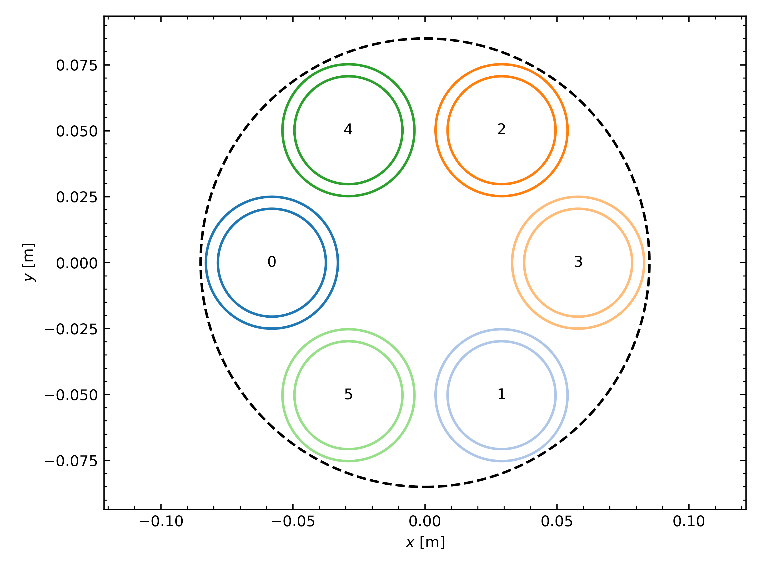
Fig 1. Triple U-tube borehole design for the benchmark of the semi-analytical model in Geoloop model with the numerical model in Geoloop.
Running the example
For running the example, either run the batch script batch_FINVOL_benchmark.py directly from your
IDE or use the CLI by:
bash
cd examples/benchmark/FINVOL_benchmark
geoloop batch-run `batch_FINVOL_benchmark.json`
455
Results
The results for the Geoloop simulations are stored in the directories output/ANALYTICAL_TU and output/FINVOL_TU.
The calculated power yield from the simulated system using both models is shown in Fig. 2. During the initial hours of system operation, the numerical model calculates a larger generated power compared to the analytical model. This is due to the transient model set-up and actually represents a more realistic short-term system performance compared to the analytical model. However, several hours after initial system operation, the calculated power yield by the different models aligns.
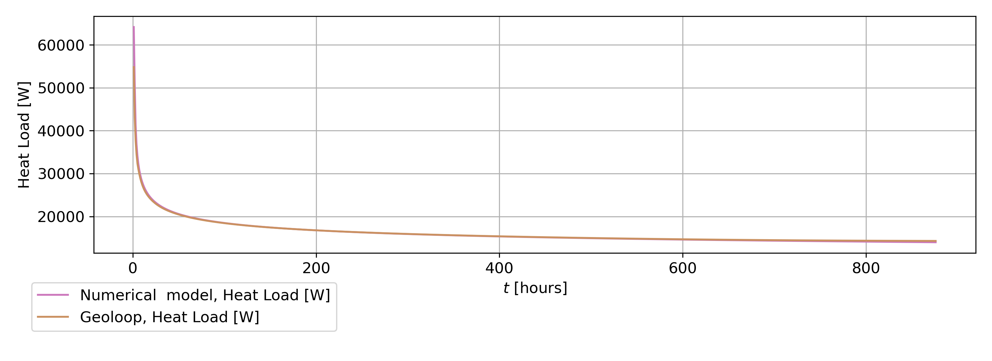
Fig. 2: Timeseries plot of generated power (\(Q\)) for the Geoloop benchmark with the numerical model.
The calculated outlet and average borehole wall temperatures that follow from the benchmark simulations is shown in Fig. 3. As consistent with the time-evolution of the generated power from the simulated system, the numerical model yields higher temperatures in the initial hours of system operation, compared to the analytical model. However, again, the models quickly align.
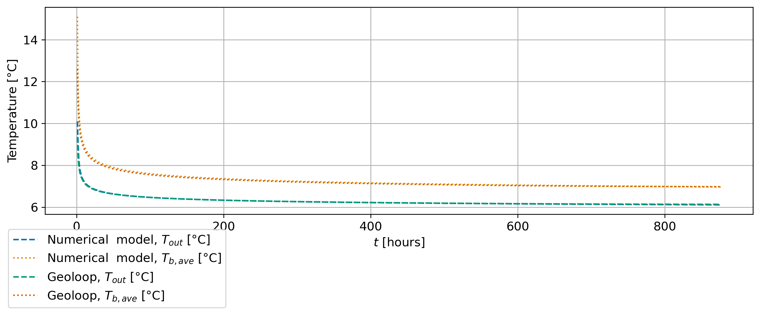
Fig. 3: Timeseries plot of outlet (\(T_{out}\)) and average borehole wall temperature (\(T_{b,ave}\)) for the Geoloop benchmark with the numerical model.
The calculated fluid temperatures over depth after one month of simulation time are shown in Fig. 4. The temperature curves for the different model types are in almost perfect agreement.
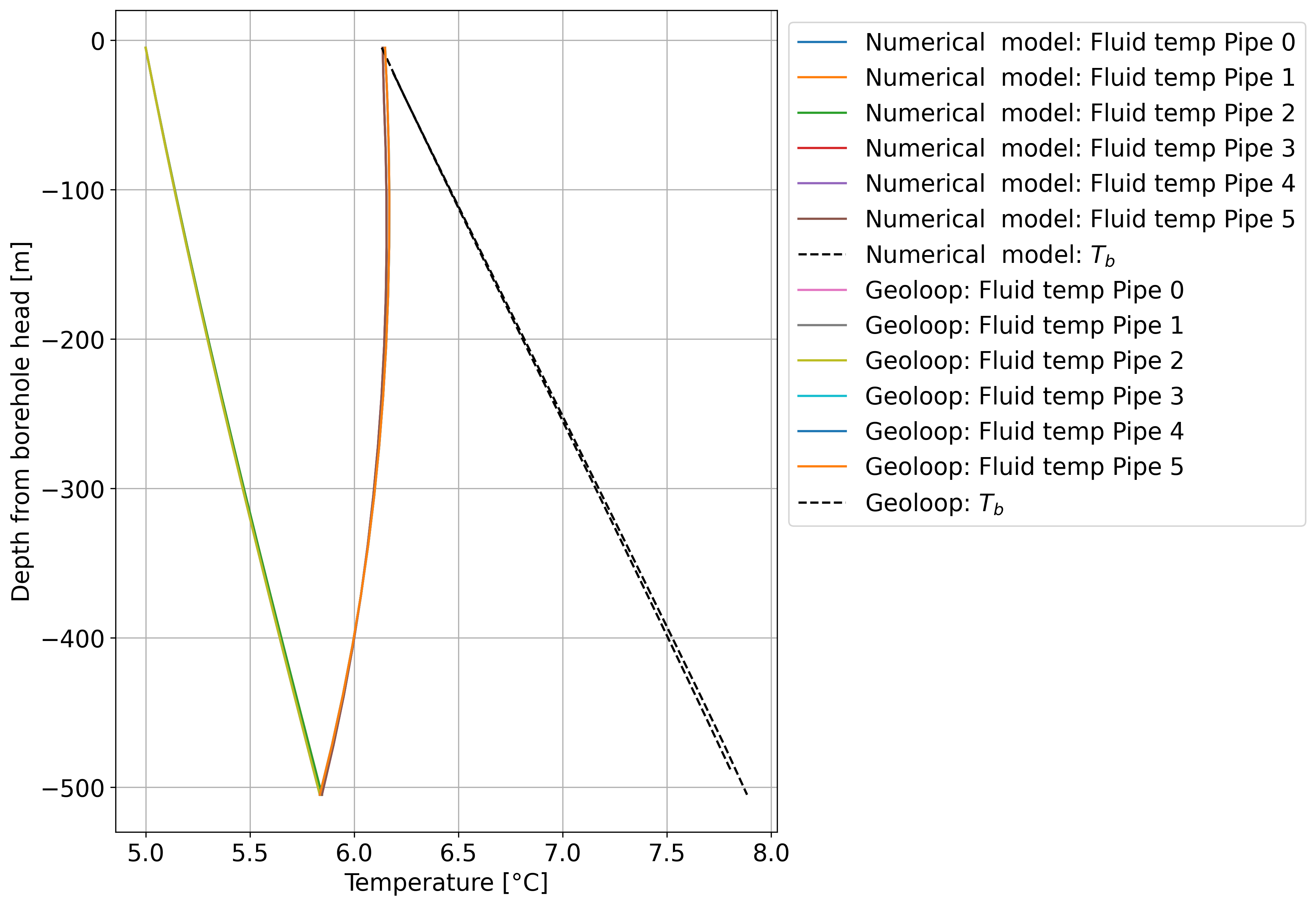
Fig. 4: Depth plot of inlet fluid (Pipe 0, 1, 2), outlet fluid (Pipe 3, 4, 5) and borehole wall (\(T_b\)) temperatures for the Geoloop benchmark with thr numerical model.
Note
The aligned results from the benchmark simulation of the semi-analytical Geoloop model and the numerical model validates the semi-analytical depth-dependent approach.
In addition to the results for the fluid and borehole wall temperatures inside the BHE system, the numerical model also calculates
the temperature field around the borehole in a radial symmetric grid. In a similar simulation as the numerical benchmark
simulation discussed above, this temperature field is stored, but for a timestep of 24 hours instead of 1 hour. The results are
stored in a separate .h5 table, and figures show the temperature field for every timestep in the directory
output/FINVOL_TU_24h_Tfield/Tfield_time/. In addition, an animation is created that shows the temperature evolution
around the borehole during the simulated BHE system operation. This is shown in Fig. 5.
Fig 5. Temperature evolution in the subsurface around a triple U-tube.
References
- Cazorla Marín, A.: Modelling and experimental validation of an innovative coaxial helical borehole heat exchanger for a dual source heat pump system, PhD, Universitat Politècnica de València, Valencia (Spain), https://doi.org/10.4995/Thesis/10251/125696, 2019.
- Cazorla-Marín, A., Montagud-Montalvá, C., Tinti, F., and Corberán, J. M.: A novel TRNSYS type of a coaxial borehole heat exchanger for both short and mid term simulations: B2G model, Applied Thermal Engineering, 164, 114500, https://doi.org/10.1016/j.applthermaleng.2019.114500, 2020.
- Cazorla-Marín, A., Montagud-Montalvá, C., Corberán, J. M., Montero, Á., and Magraner, T.: A TRNSYS assisting tool for the estimation of ground thermal properties applied to TRT (thermal response test) data: B2G model, Applied Thermal Engineering, 185, 116370, https://doi.org/10.1016/j.applthermaleng.2020.116370, 2021.