Calculation of BHE with variable maximum depth in city of Roermond
Note
The example is located in the following
working directory: geoloop/examples/lithology/roermond
This example demonstrates how a realistic depth-variable subsurface temperature and thermal conductivity profile can be incorporated in Geoloop simulations. The effect of the temperature-depth profile on the borehole performance is shown in a deterministic simulation. A stochastic simulation shows the effect of the depth-dependent subsurface thermal properties on the relation between the system performance and the maximum system depth, with uniform Monte Carlo sampling of the maximum borehole depth between 100 and 800 meters. The simulations use a fixed inlet temperature for the simulation period and therefore calculates the yearly average power yield. The inlet temperature is set to 5 °C and the flow rate is optimized conform a minimum COP of the fluid circulation pump of 15.
Subsurface thermal conductivity profile
A double U-tube is simulated, with a subsurface model as representative for the location of Roermond. In the simulation,
the thermal conductivity profiles are loaded from a pre-defined table (at output/lithology_samples_Roermond.h5),
as calculated according to the method described in the background Theory. Therefore, the index of the samples
in the stochastic simulation correspond to the index of the thermal conductivity profile in the table.
The calculated thermal conductivity-depth profile and the corresponding error range are shown in Fig. 1.
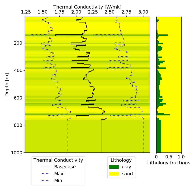
Fig. 1: Thermal conductivity-depth profile and lithological distribution down to 1000 meters, for the city of Roermond in the Netherlands.
Running the example
For running the example, either run the batch script batch_Roermond.py directly from your
IDE or use the CLI by:
Note
This example has a significant run-time (>2h).
Results
The Lithology command in the batch_Roermond.json file runs the lithology module with the provided configuration file.
Since the flag read_from_table in the configuration of the lithology module is set to true, the table with subsurface
thermal conductivity profiles must be pre-defined. Running the Lithology command creates the figure to visualize the
subsurface model, in Fig. 1.
In case the read_from_table flag is set to false, the set of thermal conductivity profiles is calculated from the
subsurface lithology data linked in the configuration file.
The effect of the temperature-depth profile on the fluid temperatures and borehole wall temperature of the simulated system are shown in Fig. 2.
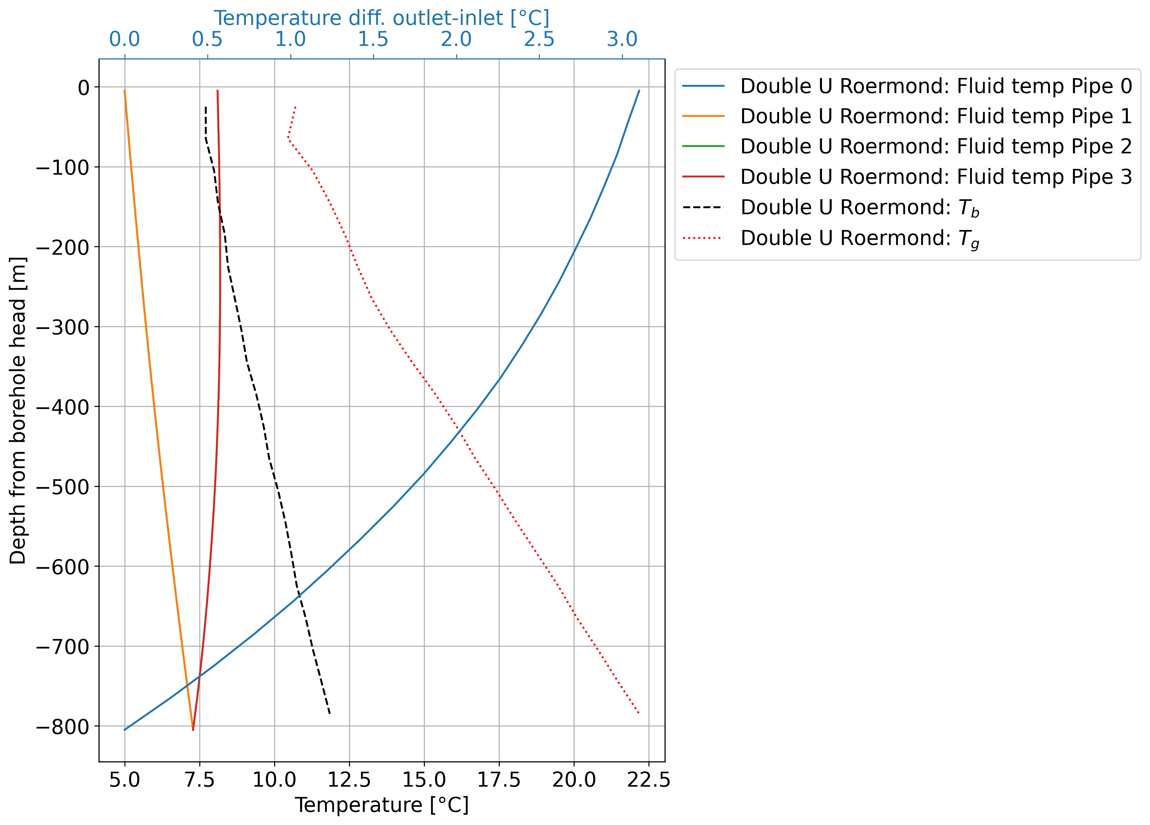
Figure 2: Fluid, borehole wall and subsurface temperature of the simulated double U-tube BHE system in Roermond, down to 800 meters and after 100 hours of operation.
The relation between maximum system depth and average power yield in the first year of operation, at the location of Roermond, is shown in Fig. 3. The scattered nature in the plotted datapoints derives from the uncertainty range applied to the subsurface properties in the calculation of the thermal conductivity profiles. The non-linear increase in power yield with depth is related to the depth-dependency in the subsurface properties, and shows how the potential for deeper BHE systems is fostered when considering subsurface heterogeneity in predictions of the system performance.
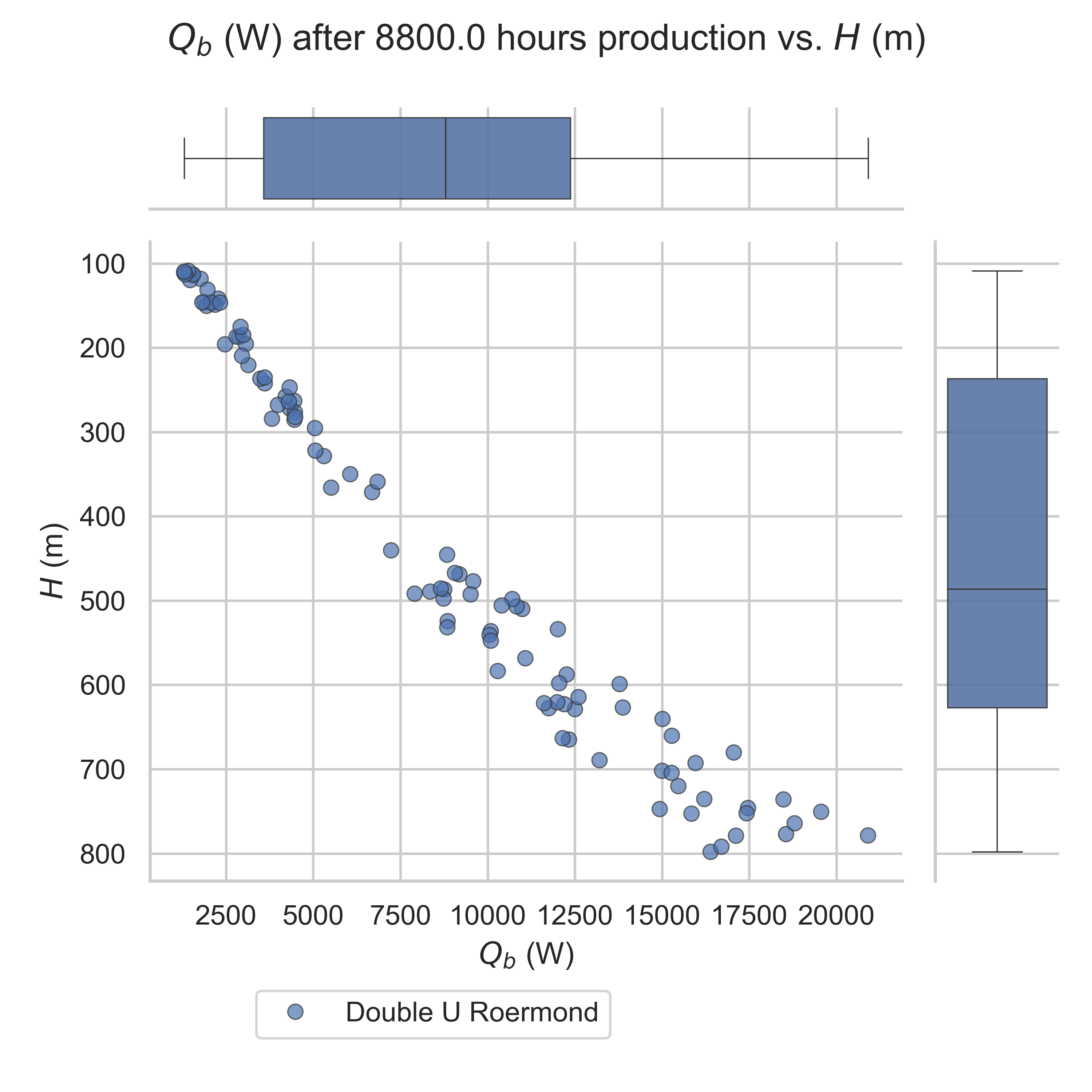
Fig. 3: Relation between average generated power (\(Q\)) in the first year of operation and the maximum depth (\(H\)) of a double U-tube BHE system in Roermond.