Calculation of a rectangular BHE field for cooling in the Middle East
Note
The example is located in the following
working directory: geoloop/examples/bore_field/ME_cooling
This example demonstrates the use of the main commands
SingleRunSim and Plotmain to calculate and display the results for a borehole field with vertical boreholes for cooling in the Middle East.
The concept of effective bore field and its numerical solution by pygfunction is detailed by
(Cimmino & Cook, 2022). The solution assumes a uniform borehole wall temperature and a parallel inlet and outlet temperature profile.
The cooling demand is based on a total energy demand generated from Ninja Renewables (Pfenninger & Staffell, 2016; Staffell & Pfenninger, 2016)
for a city in the middle east for the year 2018. The cooling demand is also displayed in a figure using the Loadprofile command.
In addition, in using the pre-defined load profile, the flow rate is scaled such that the ratio of the required pumping power
to the generated power (or the COP of the fluid circulation pump) is constant.
The borehole field consists of 25 vertical boreholes with a borehole length of 150 m and a borehole diameter of 0.14 m. The boreholes are arranged in a 5x5 grid with a spacing of 25 m. The boreholes are equiped with parallel double U-tubes, deploying water as working fluid.
The borehole field is simulated for a period of 10 years with a time step of 1 hour.
Running the example
For running the example, either run the batch script batch_me.py directly from your
IDE or use the CLI by:
Results
In the command Loadprofile the cooling demand is loaded from a csv file generated by Ninja renewables ninja_demand_me.csv and
scaled by lp_scale parameter. The resulting cooling demand is displayed as a figure in ninja_demand_me.png (Fig. 1).
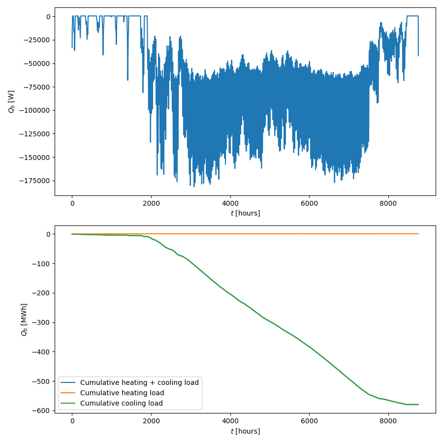
Fig. 1: Heat/cold demand for a city in the middle east in year 2018, scaled by -200 (cooling is negative).
For a yearly analysis it is easier to smooth out the oscillatory character of the hourly-variable load profile. Therefore, a smoothing is applied to obtain monthly load values (see Fig. 2), that are then used in the simulation of the borehole field.
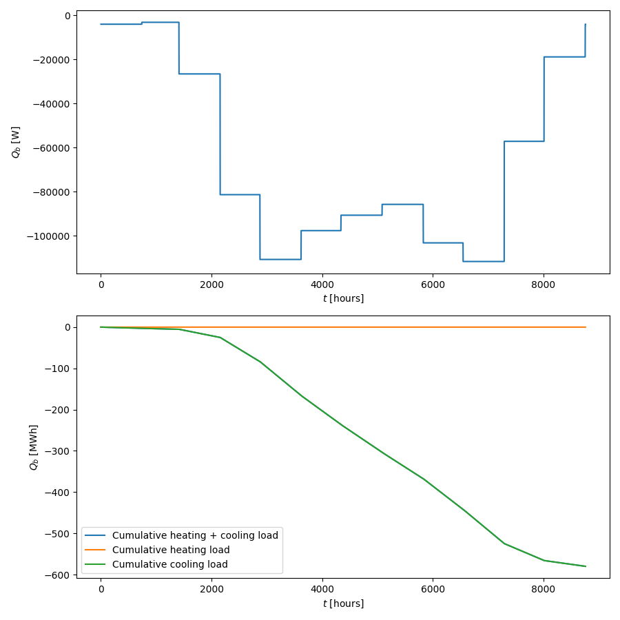
Fig. 2: Ninja demand for a city in the middle east in year 2018 scaled to -200 (cooling is negative) and smoothed to monthly load values.
The simulation results are stored in the directory output/me_du and contain the borehole field geometry and borehole tubing layout as output from
SingleRunSim (Fig. 3 and Fig. 4).
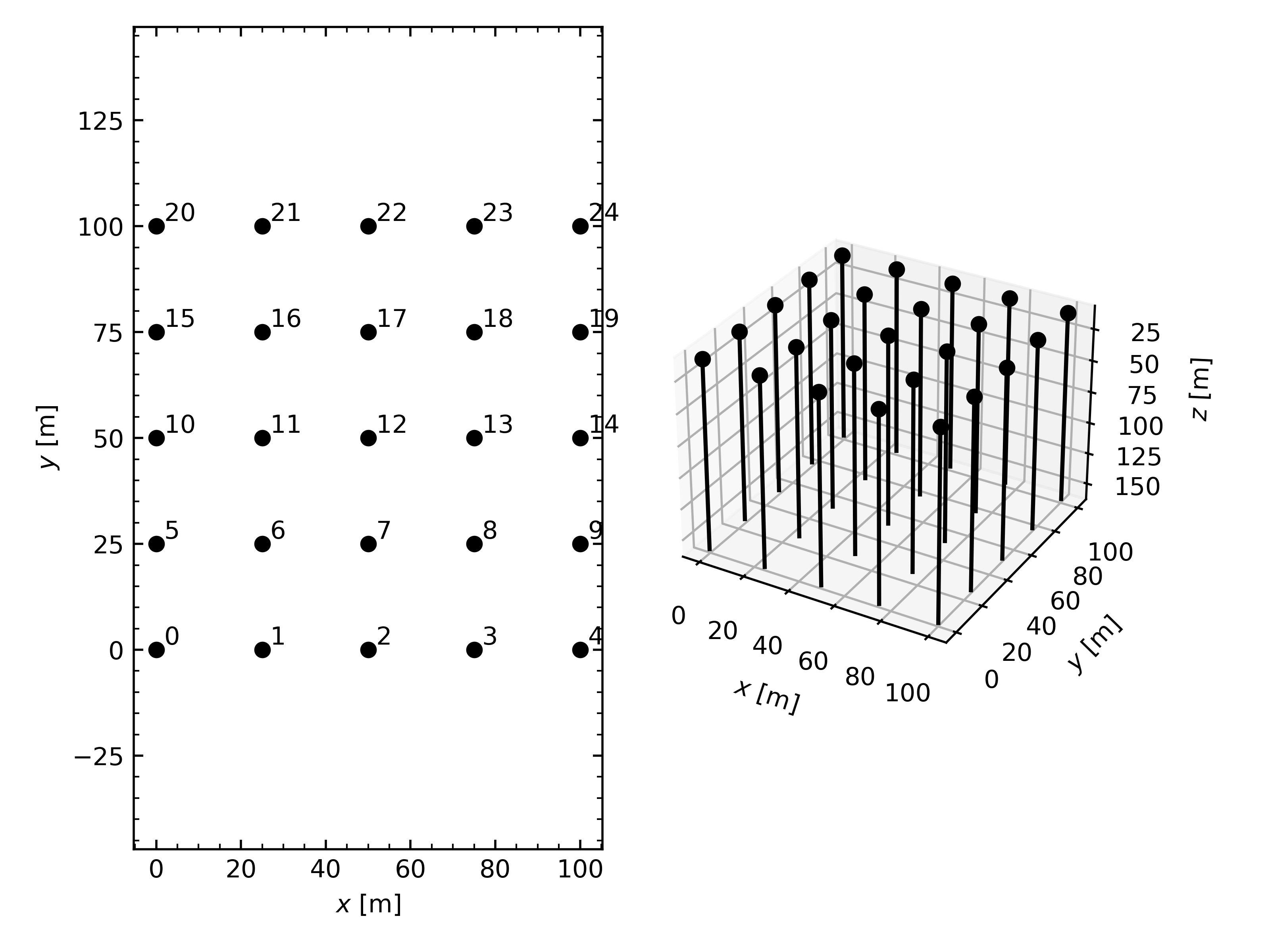
Fig. 3: Layout of the square bore field for cooling in the Middle East.
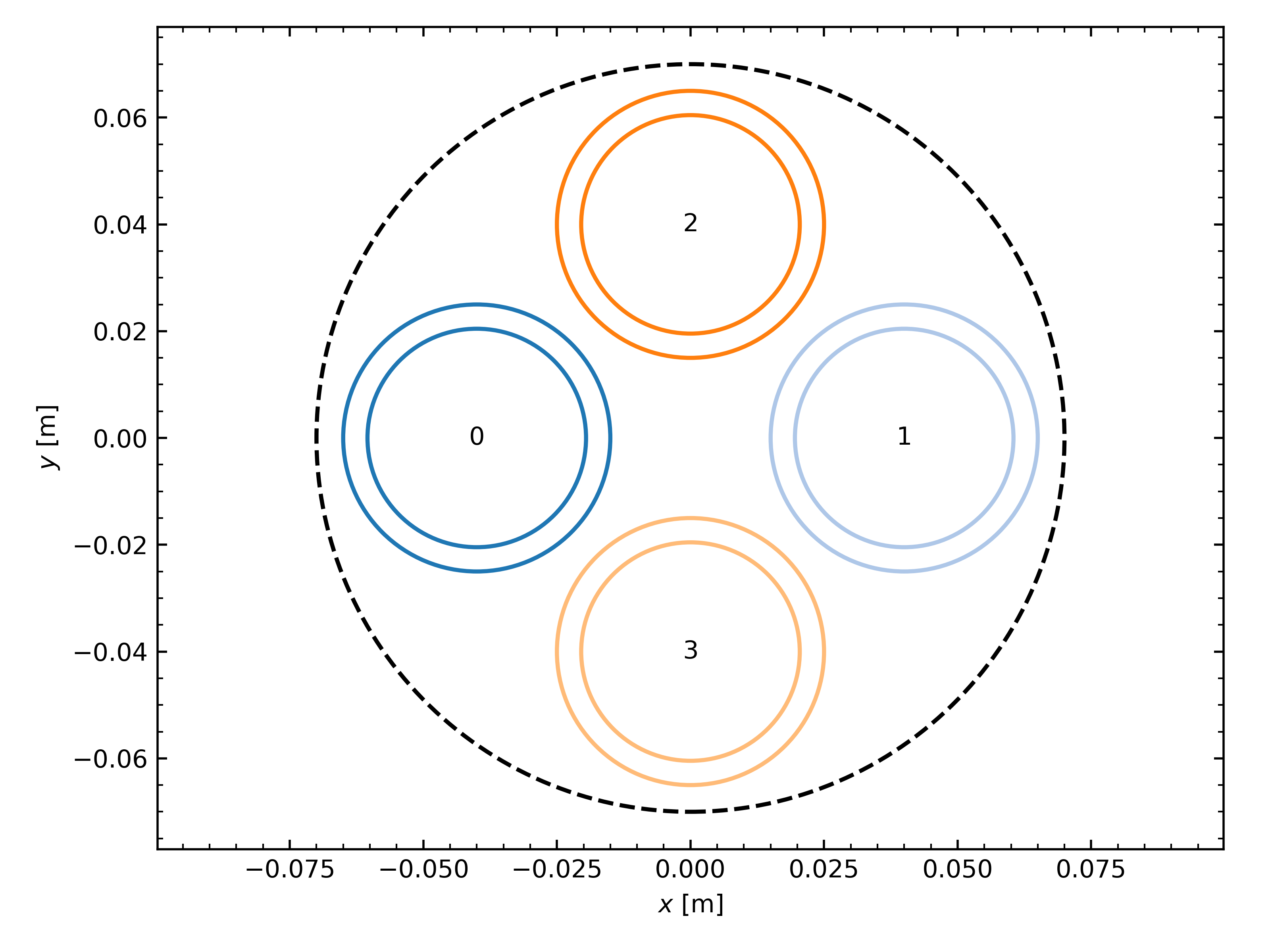
Fig. 4: design of the double utubes in the boreholes for cooling in the Middle East.
Other results have been visualized by running the Plotmain command (Fig. 5).
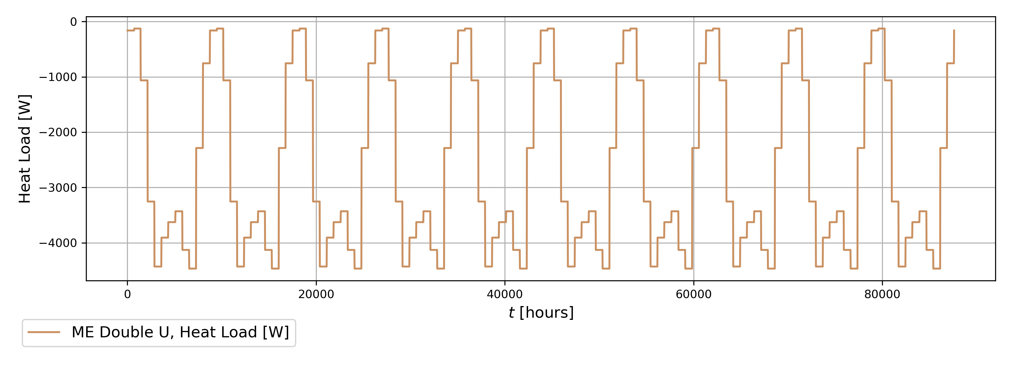
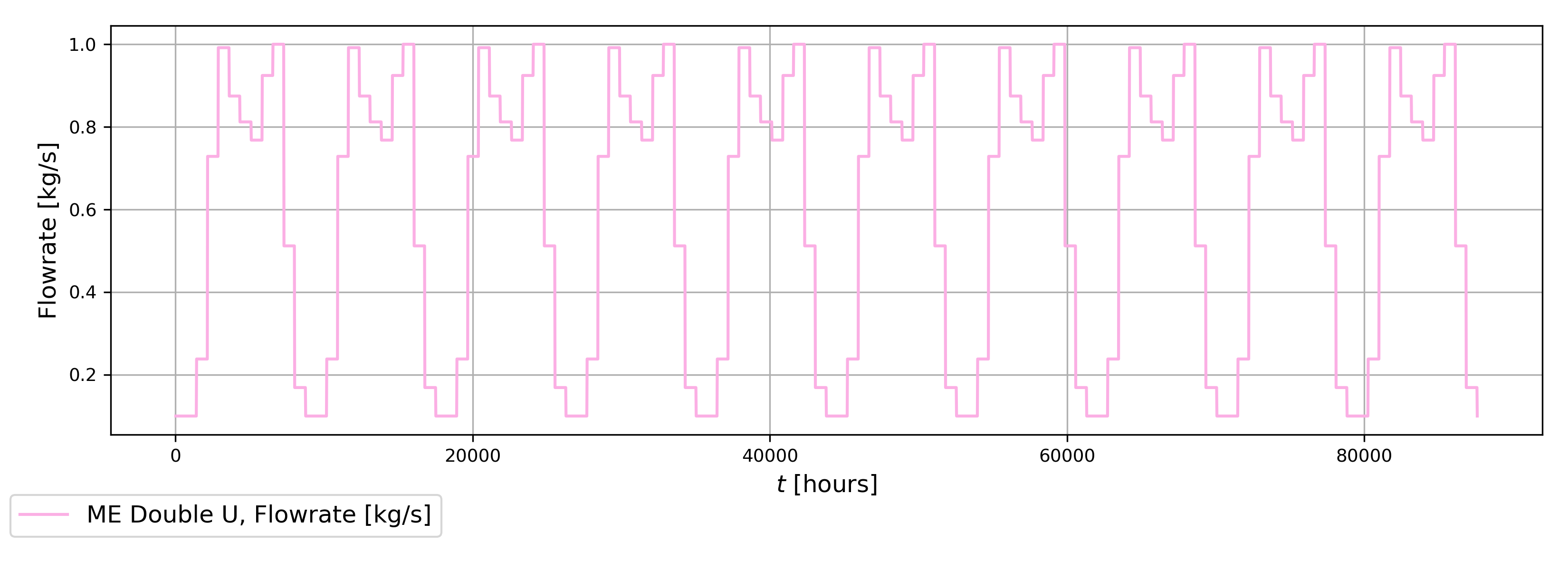
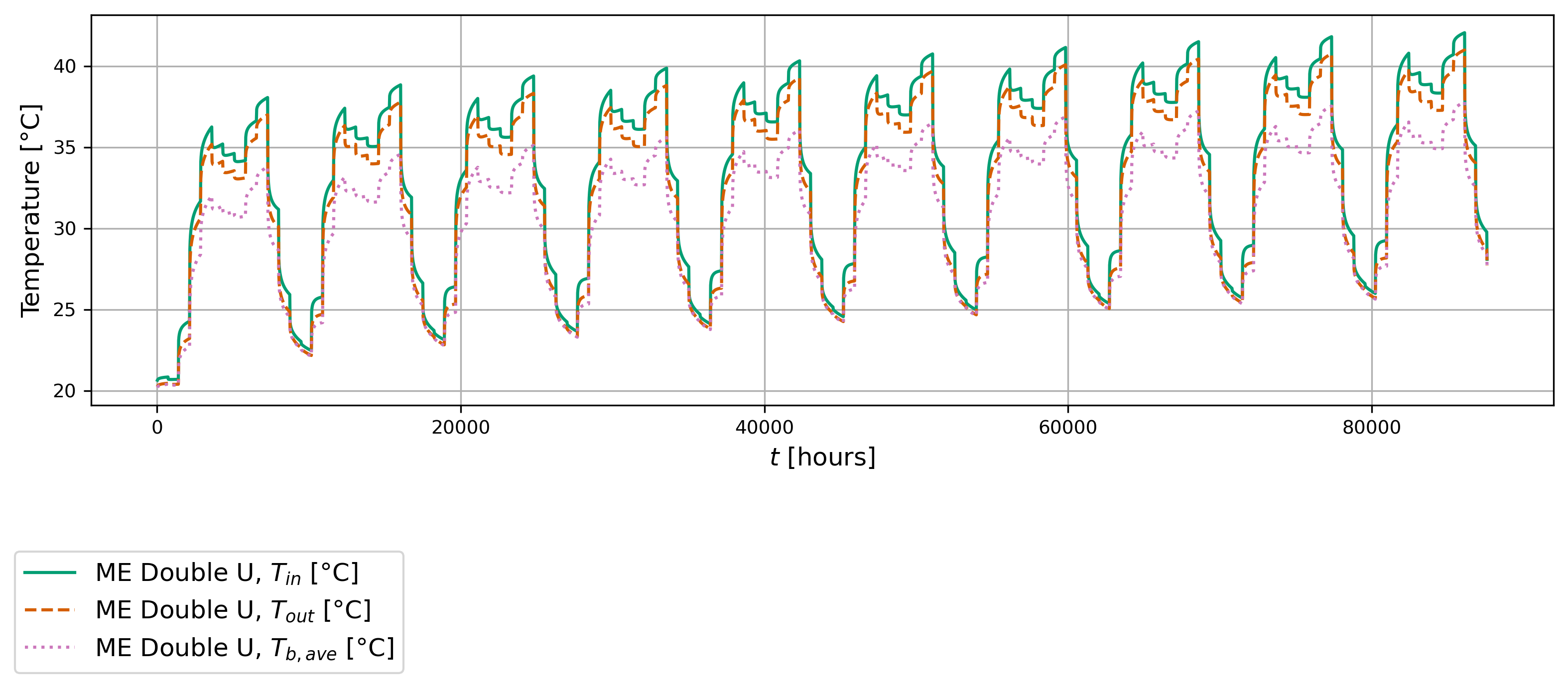
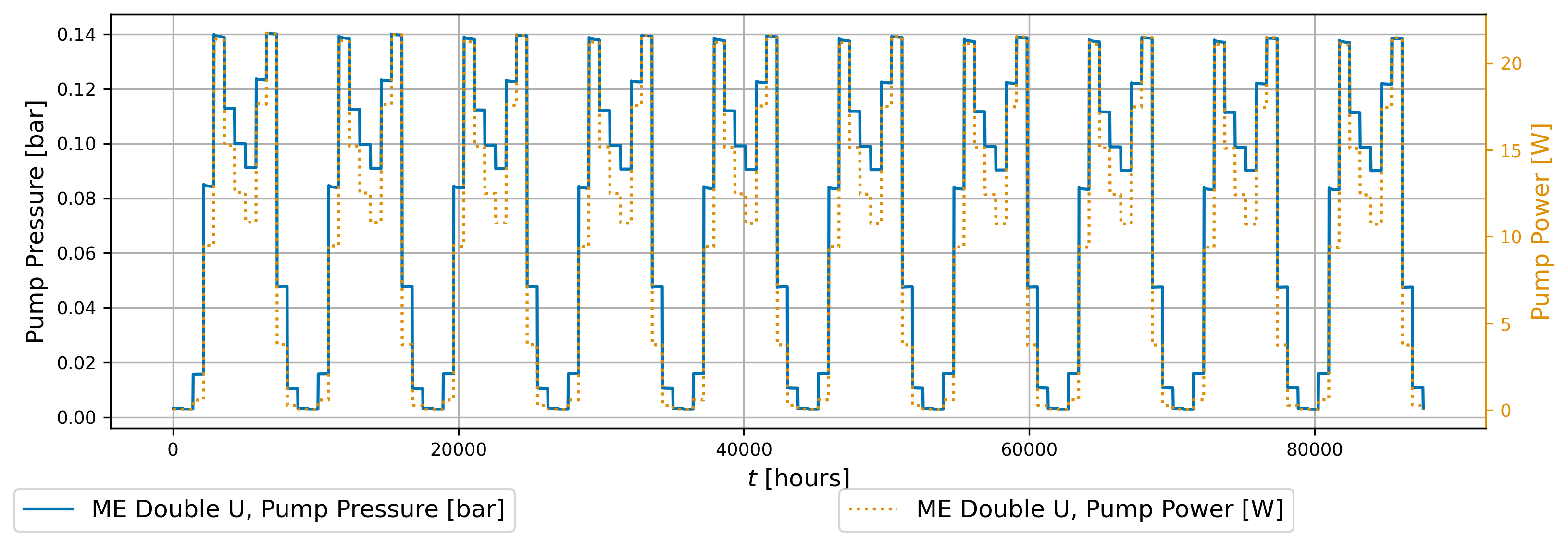
Fig. 5: Timeseries plot of the square bore field, (\(Qb\)) heat demand for each borehole in the field, (\(flowrate\)) mass rate and sign of flow, inlet temperature (\(T_{in}\)), outlet temperature (\(T_{out}\), borehole wall temperature (\(T_b\)), pumping pressure (\(dploop\)) and required pumping power (\(qloop\)).
References
- Cimmino, M. and Cook, J.: pygfunction 2.2: New features and improvements in accuracy and computational efficiency, in: Proceedings of the IGSHPA Research Track 2022, International Ground Source Heat Pump Association, https://doi.org/10.22488/okstate.22.000015, 2022.
- Pfenninger, S. and Staffell, I.: Long-term patterns of European PV output using 30 years of validated hourly reanalysis and satellite data, Energy, 114, 1251–1265, https://doi.org/10.1016/j.energy.2016.08.060, 2016.
- Staffell, I. and Pfenninger, S.: Using bias-corrected reanalysis to simulate current and future wind power output, Energy, 114, 1224–1239, https://doi.org/10.1016/j.energy.2016.08.068, 2016.