Benchmark of Geoloop with the pygfunction python package, for a single and a double U-tube
Note
The example is located in the following working directory: geoloop/examples/benchmark/PYG_benchmark
This example demonstrates the benchmark of the semi-analytical depth-dependent Geoloop model with the standard implementation of g-funtions in the pygfunction python package functionality (Cimmino & Cook, 2022), for a single and double U-tube design. The option of using the standard pygfunction package is incorporated in the Geoloop package.
The same BHE design, of a double and single U-tube respectively, was simulated using both model types. Since the pygfunction package does not allow for depth-dependent (subsurface) properties, the benchmark simulations include fixed values for the subsurface temperature and thermal conductivity over depth. The pygfunction package by default includes one model segment over depth. In the Geoloop model, the number of model segments was set to 10, to illustrate how the depth-dependent solution yields the same results as the standard implementation of g-functions.
The performance calculations target the fluid temperatures, given a constant heat load over time. The flow rate was fixed at a constant value during the simulated time and the system performance was calculated for a simulation period of 10 years.
For both benchmark simulations, BHE design and simulation parameters are provided in the table below and Fig. 1 and 2.
| Simulation parameter | Single U-tube | Double U-tube |
|---|---|---|
System length (H) |
100 m | 500 m |
Buried depth (D) |
0 m | 0 m |
Grout thermal conductivity (k_g) |
0.844 W/mK | 0.844 W/mK |
Working fluid (fluid_str) |
water | water |
Borehole radius (r_b) |
0.07 m | 0.07 m |
Outer pipe radius (r_out) |
0.02 m | 0.02 m |
SDR-value (SDR) |
11 | 11 |
Pipe thermal conductivity (k_p) |
0.41 W/mK | 0.41 W/mK |
Subsurface temperature (T_g) |
11 °C | 15 °C |
Subsurface bulk thermal conductivity (k_s) |
2.4 W.mK | 2.4 W/mK |
Heat load (Q) |
1000 W | 5000 W |
Flowrate (m_flow) |
0.3 kg/s | 1 kg/s |
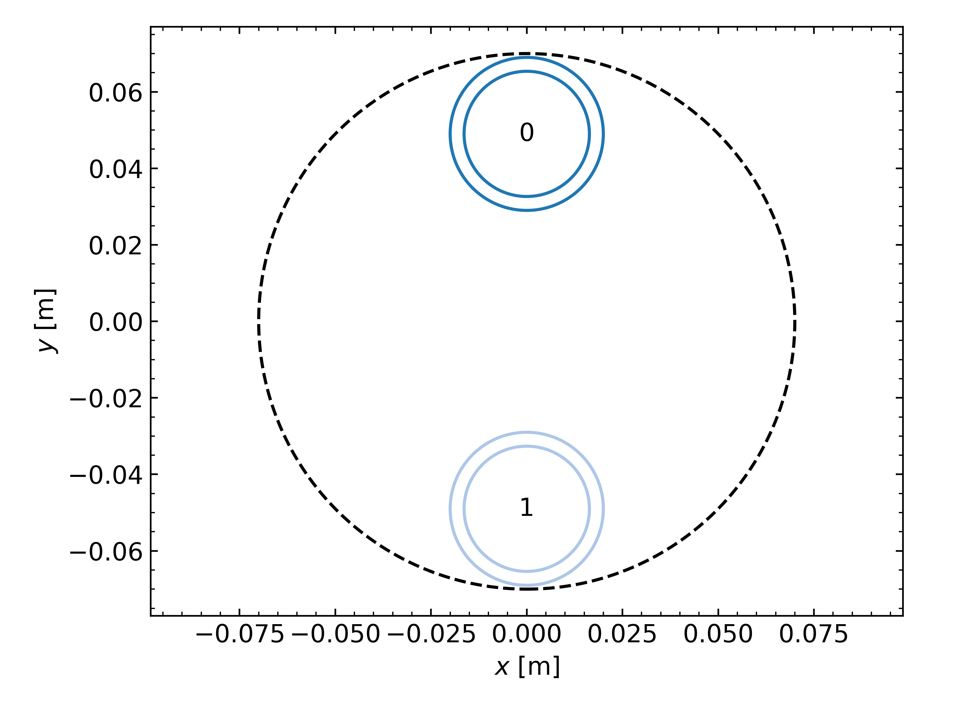
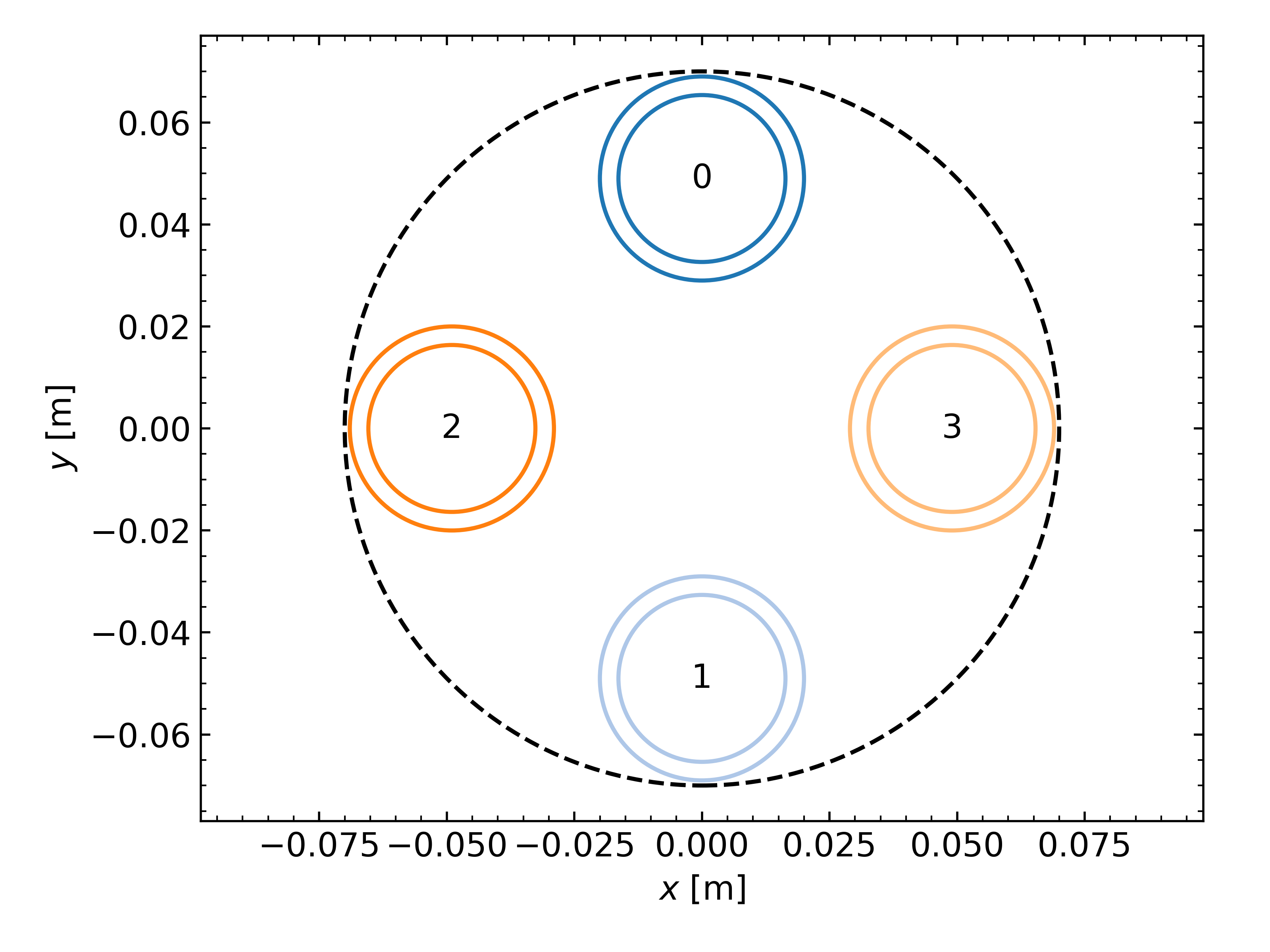
Fig. 1 & 2: Single U-tube (top) and double U-tube (bottom) borehole design for the benchmark simulations.
Running the example
For running the example, either run the batch script batch_PYG_benchmark.py directly from your
IDE or use the CLI by:
Results
The simulation results are stored in the output/PYG_* and output/ANALYICAL_* directories.
Single U-tube
The results of the benchmark simulation for the single U-tube are shown in Fig. 3 and 4. Fig. shows the calculated inlet,
outlet and average borehole wall temperatures over time and Fig. 4 shows the fluid and borehole wall temperatures over depth
after one year of operation. In all plots, the results of both simulations are plotted together, by setting the newplot flag
in the plotting configuration to false (see Manual).
The curves from the semi-analytical depth-dependent model in Geoloop and the standard implementation of g-functions are in perfect agreement in the plots.
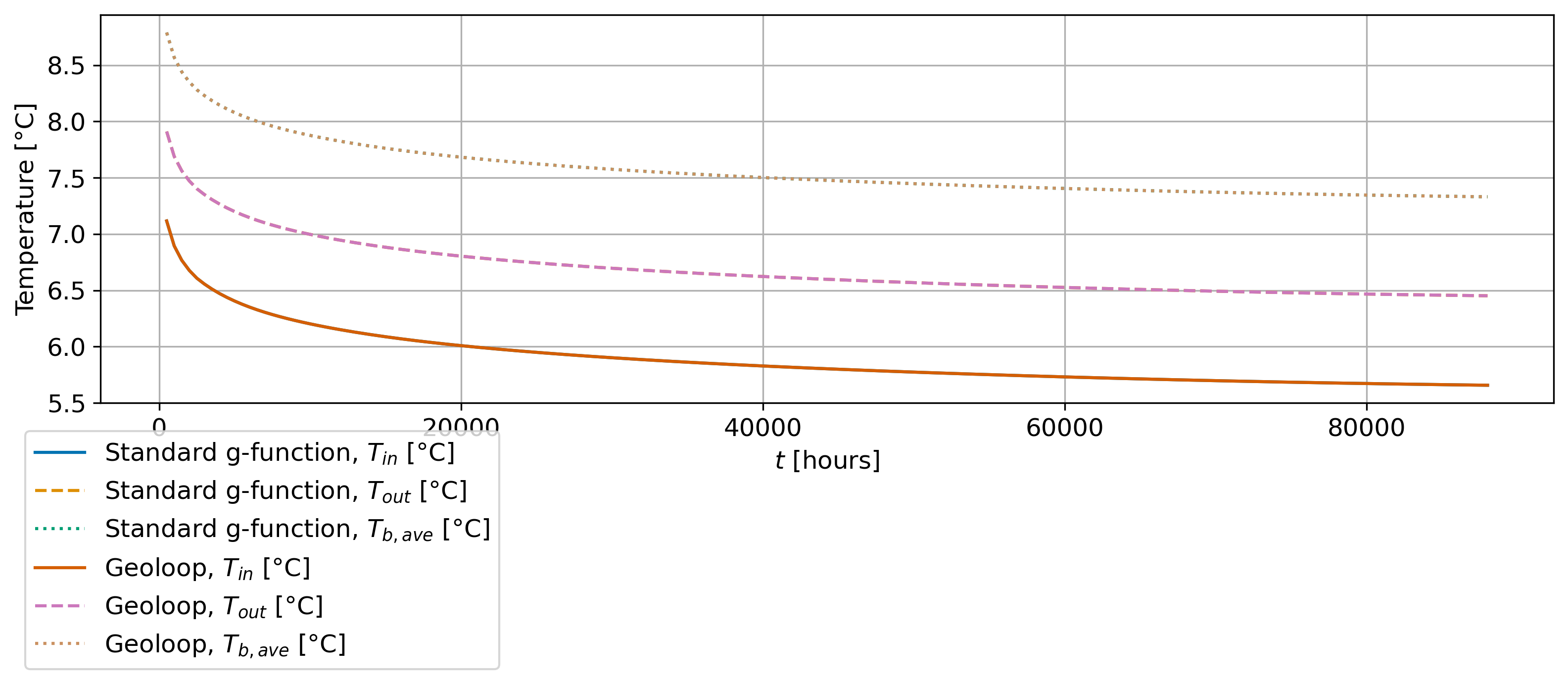
Fig. 3: Timeseries plot of inlet (\(T_{in}\)), outlet (\(T_{out}\)) and average borehole wall temperature (\(T_{b,ave}\)) for the Geoloop benchmark simulations of the single U-tube borehole design. Please note that standard g-function and geoloop outcomes are in perfect agreement.
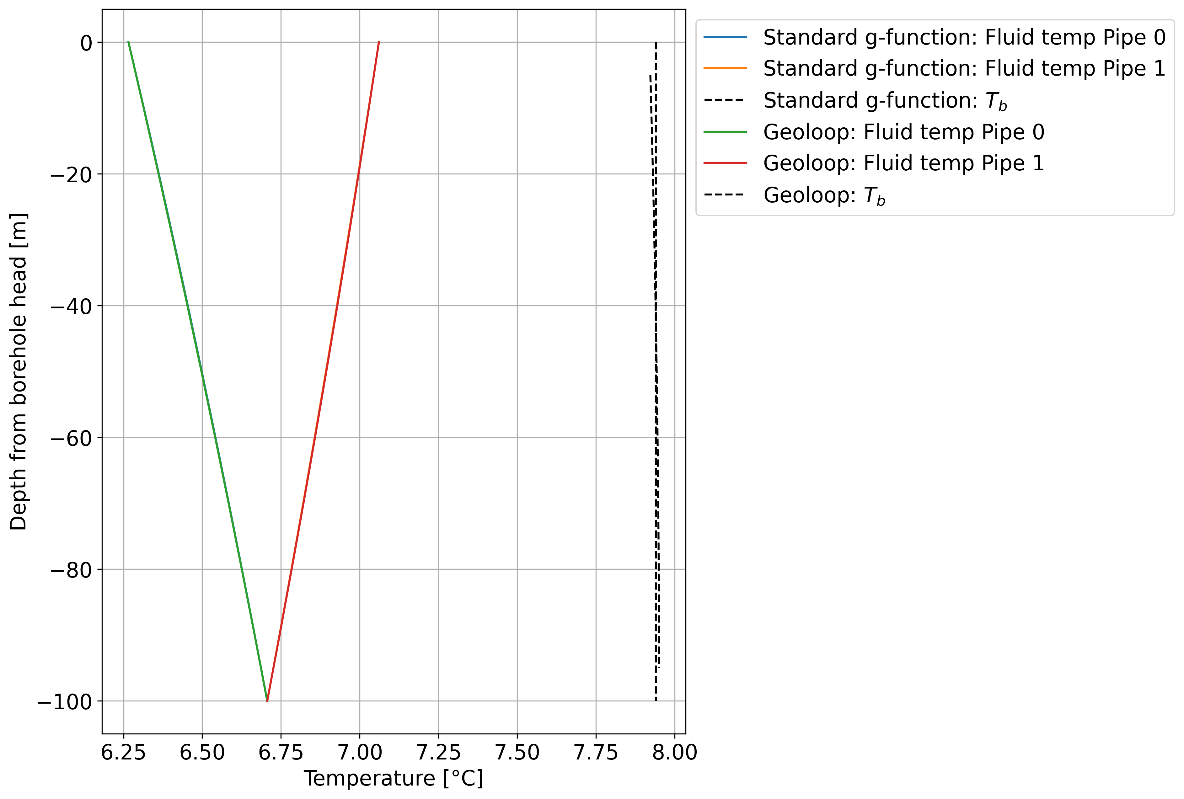
Fig. 4: Depth plot of inlet fluid (Pipe 0), outlet fluid (Pipe 1) and borehole wall (\(T_b\)) temperatures for the Geoloop benchmark simulations of the single U-tube borehole design. Please note that resulting temperatures of standard g-function and geoloop are in perfect agreement.
Double U-tube
The results of the benchmark simulations for the double U-tube are shown in Fig. 3 and 4. Fig. shows the calculated inlet, outlet and average borehole wall temperatures over time and Fig. 4 shows the fluid and borehole wall temperatures over depth after one year of operation.
Both models yield the same BHE inlet and outlet temperatures and average borehole wall temperatures. Therefore, the benchmark is successful. However, there is a slight difference between the fluid and borehole temperatures over depth, calculated by the two models. This is caused by model the set-up with multiple depth-segments in the Geoloop model, and is also reflected in the calculated temperature field inside the borehole, as shown in Fig. 5 and 6.
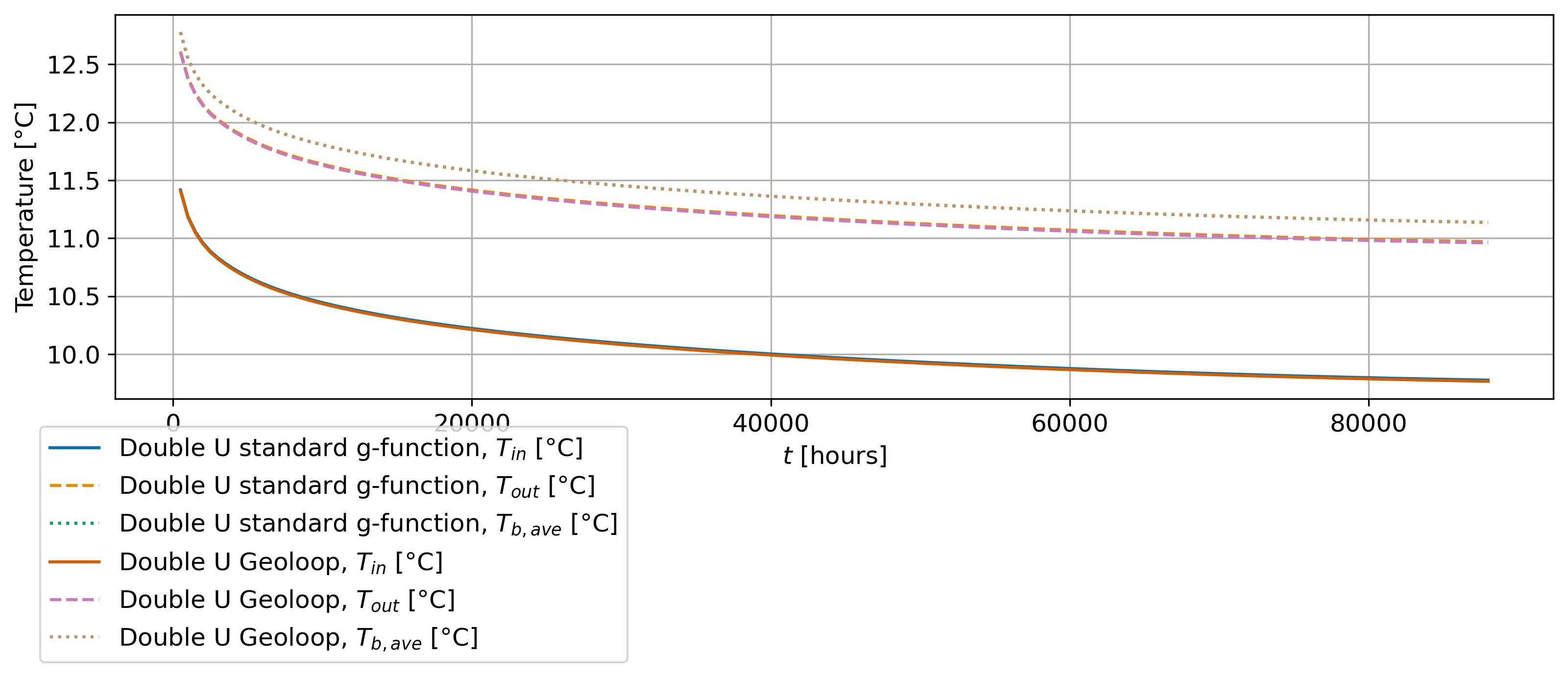
Fig. 3: Timeseries plot of inlet (\(T_{in}\)), outlet (\(T_{out}\)) and average borehole wall temperature (\(T_{b,ave}\)) for the Geoloop benchmark with pygfunction, for the double U-tube borehole design. Please note that resulting temperatures of standard g-function and geoloop are in perfect agreement.
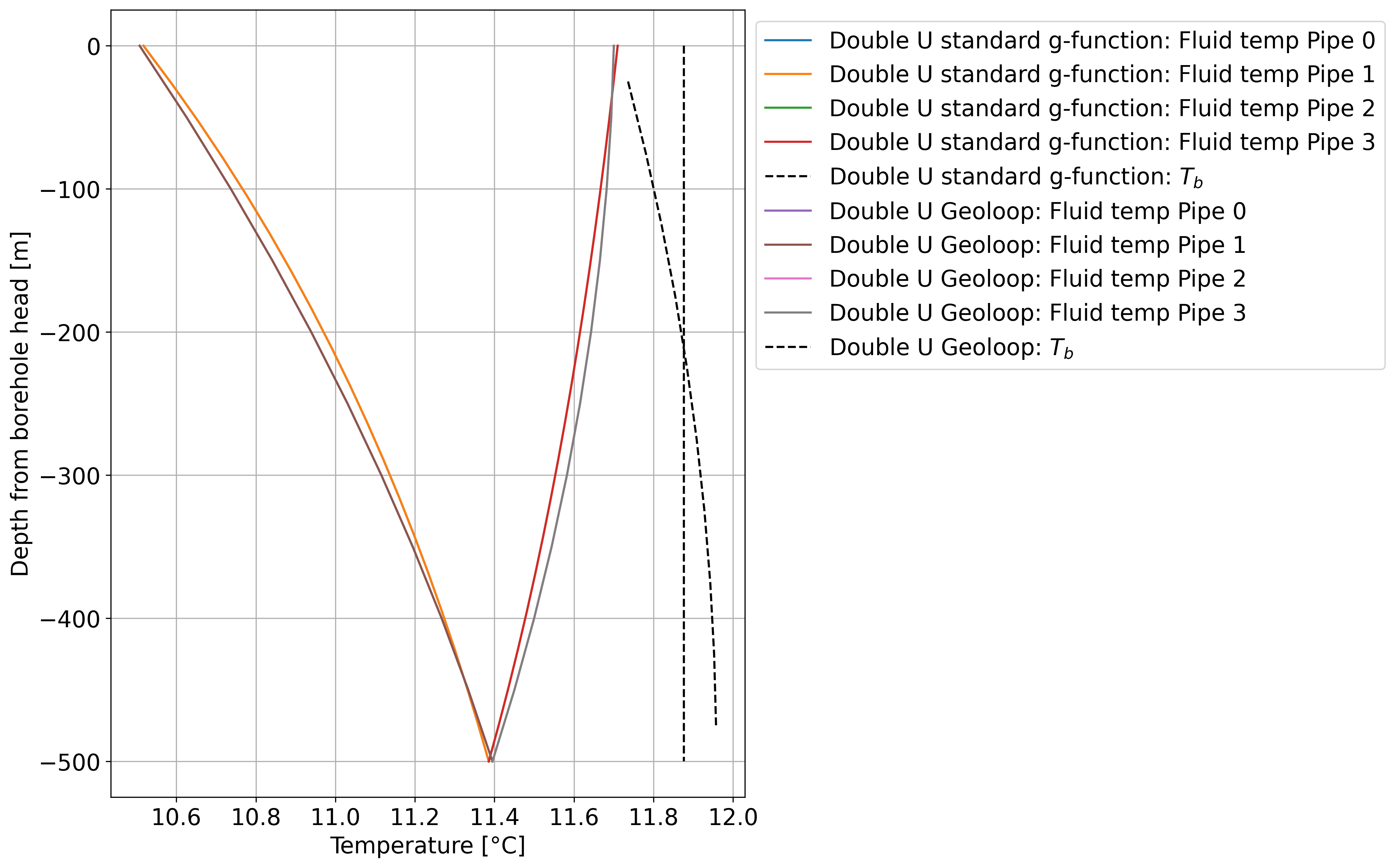
Fig. 4: Depth plot of inlet fluid (Pipe 0, 1), outlet fluid (Pipe 2, 3) and borehole wall (\(T_b\)) temperatures for the Geoloop benchmark with pygfunction, for the double U-tube borehole design.
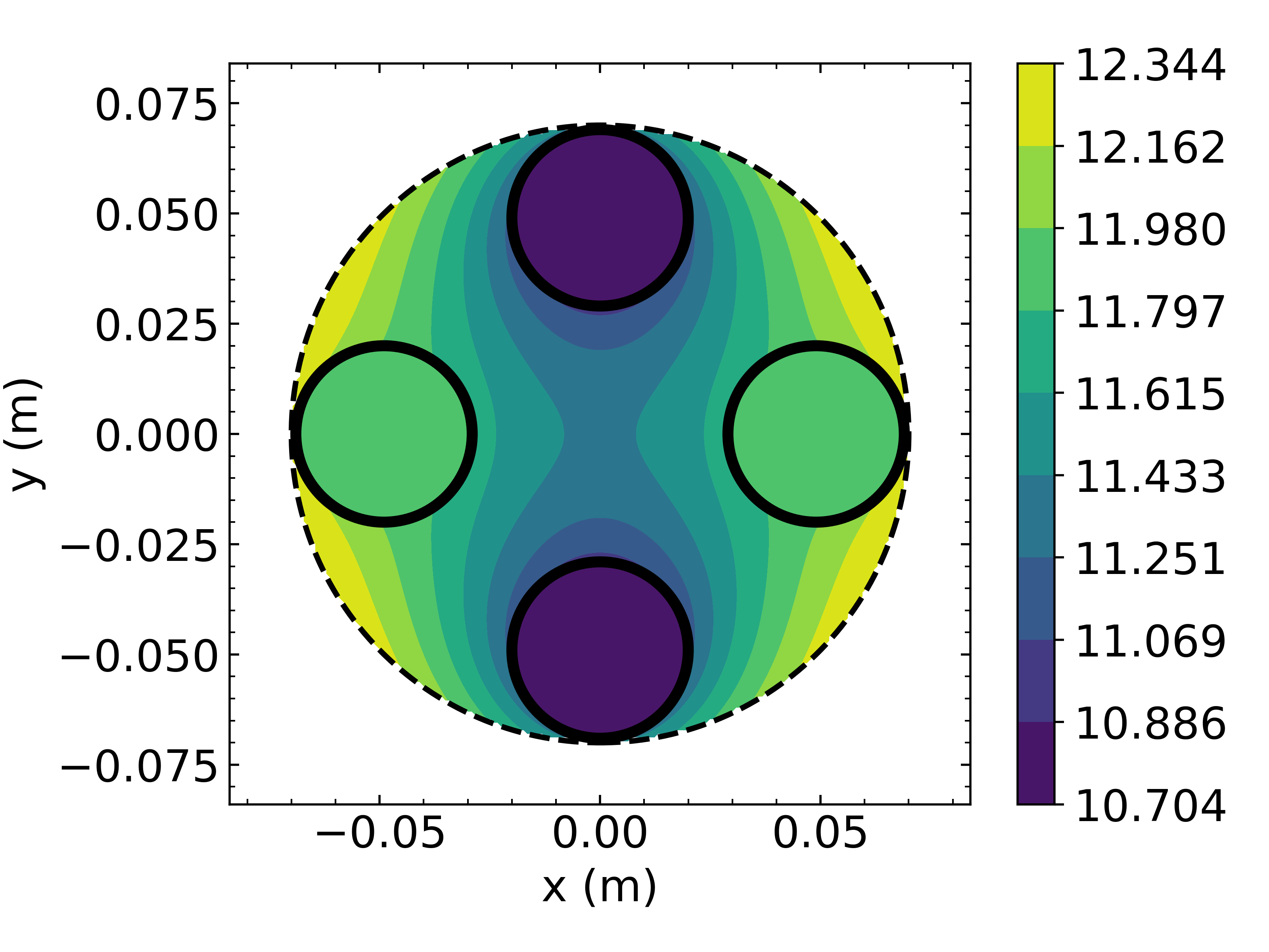
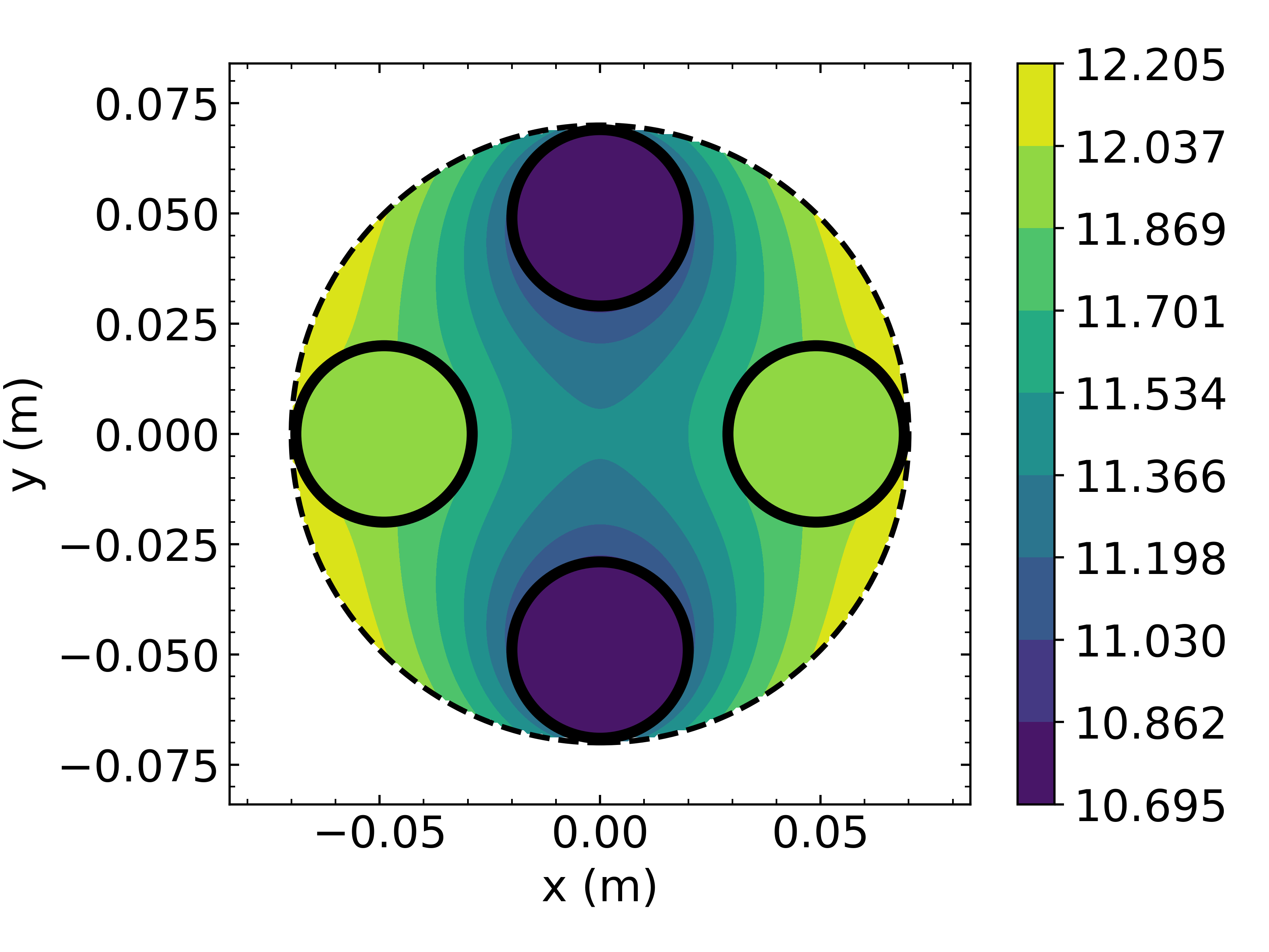
Fig. 5 & 6: Temperature (°C) inside borehole with a Double U-tube after half a year of operation, calculated with the standard g-function method (top) and by the semi-analytical Geoloop model (bottom).
Note
The results from the benchmark simulation of the semi-analytical model in Geoloop and the standard implementation of g-functions validates the semi-analytical modelling approach that allows for a depth-dependent BHE design and subsurface model.
References
- Cimmino, M. and Cook, J.: pygfunction 2.2: New features and improvements in accuracy and computational efficiency, in: Proceedings of the IGSHPA Research Track 2022, International Ground Source Heat Pump Association, https://doi.org/10.22488/okstate.22.000015, 2022.