Optimization of a coaxial BHE
Note
The example is located in the following
working directory: geoloop/examples/optimization
This example demonstrates how the simulated BHE design can be optimized for a maximum power yield within the specified operational boundary conditions. Therefore, a coaxial heat exchanger down to 500 meters is simulated twice; once to determine to optimal flowrate and design with an insulation layer around the outlet (inner) pipe and once to determine the optimal flowrate in combination with the optimal radius of the inner pipe. In both simulations, the performance of the BHE is iteratively calculated, while varying the optimized input parameters conform the specified sampling method and value ranges. This process is repeated until a model configuration is obtained that yields the maximum power while respecting the operational boundary condition(s) of a minimum COP and/or the imposed pumping pressure. Both simulations run for a year, with a constant inlet temperature of 5 °C.
Running the example
For running the example, either run the batch script batch_COAX_optimization.py directly from your
IDE or use the CLI by:
Results
Optimal flow rate and pipe insulation
In the first simulation, the simulated coaxial BHE is shown in Fig. 1. The insulation layer, for which the maximum depth along the inner pipe is optimized, represents a foam material with a thermal conductivity similar to that of air and it comprises half the inner pipe thickness.
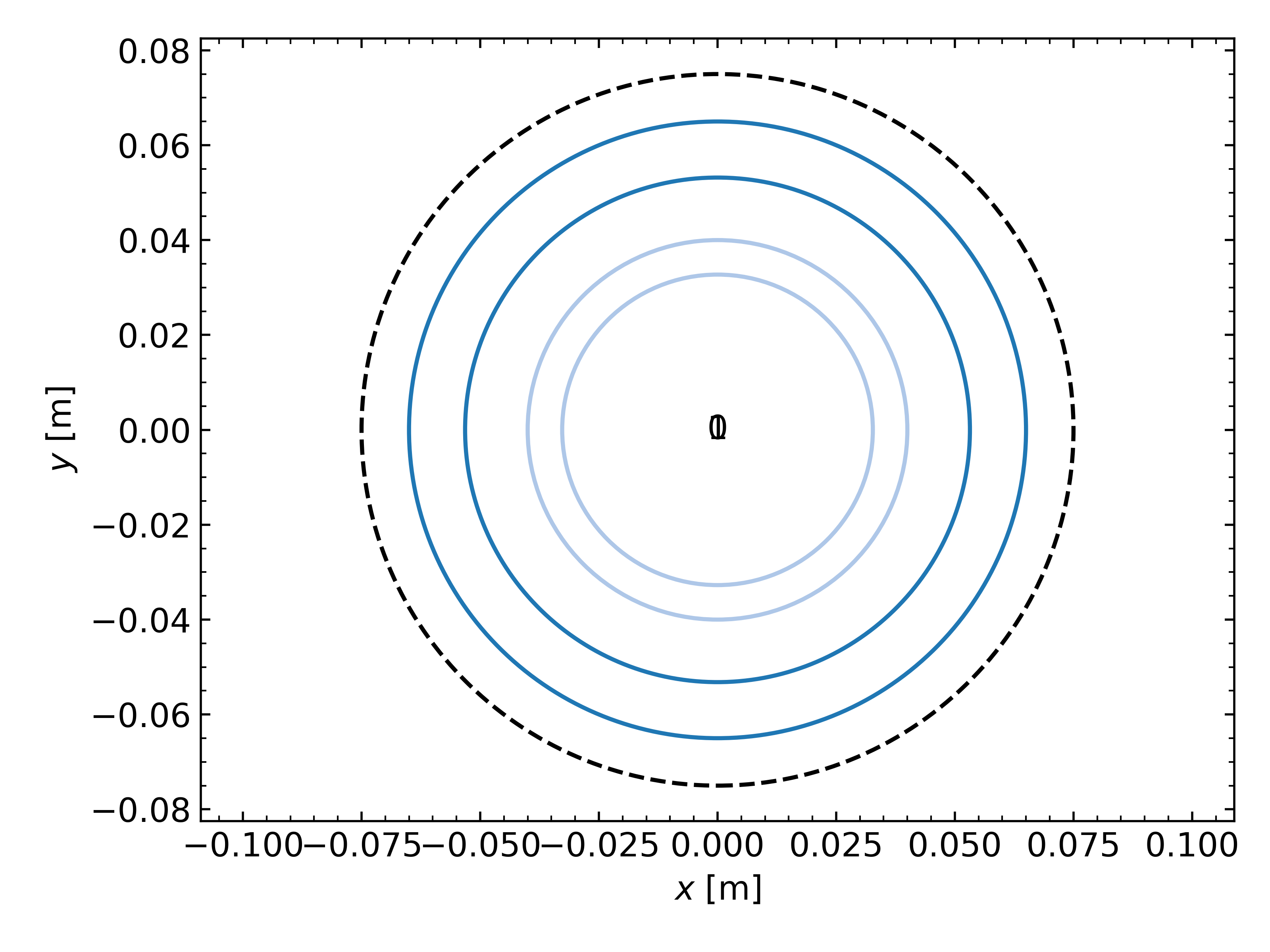
Fig. 1: Cross-section of the BHE design in the optimization simulation of an insulation layer in the inner pipe for maximum power yield of the system.
Both the flowrate and the design of the insulation layer are optimized under the condition of a minimum COP of the fluid circulation pump of 20.
The results yield an optimal flowrate of about 2.5 kg/s at a pumping pressure of about 1.7 bar, for a BHE design with the pipe insulation layer down to about 380 meters. This layer limits heat loss during upward transport of the working fluid, as is reflected in the fluid temperatures over depth after half a year of operation (see Fig. 2).
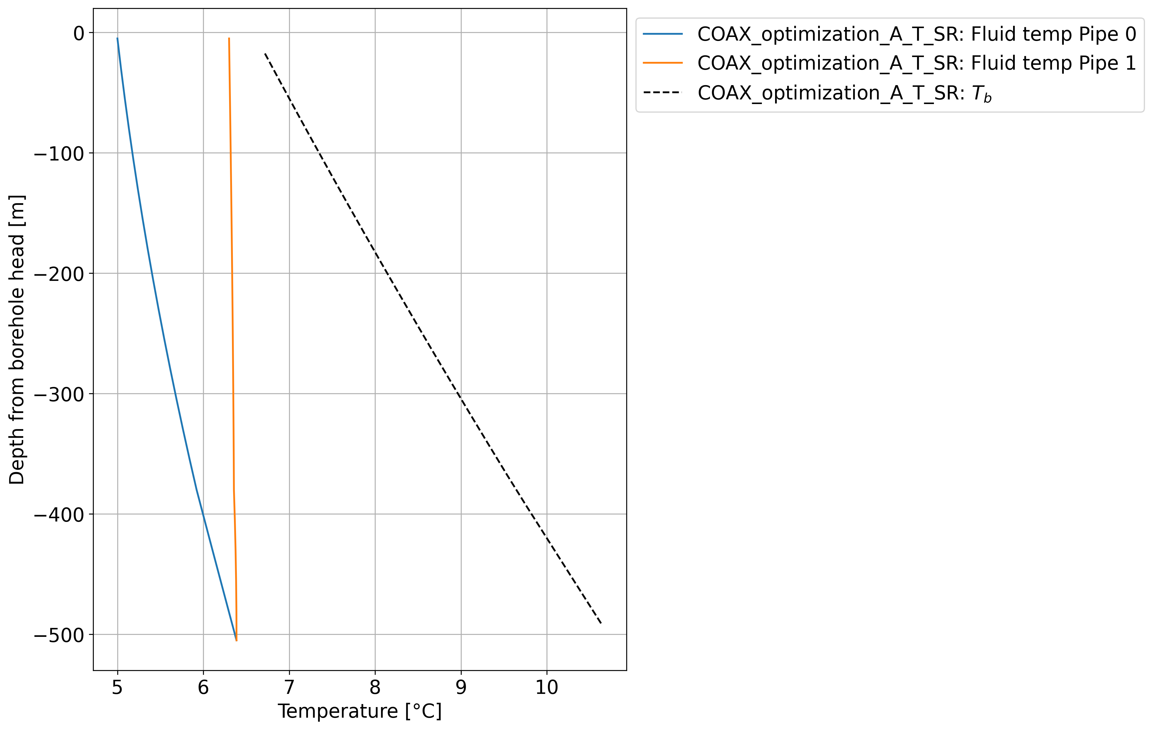
Fig. 2: Fluid and borehole wall temperatures after half a year of operation of the coaxial BHE with an optimized flow rate and pipe insulation design.
The power yield that follows from the simulation is shown in Fig. 3.
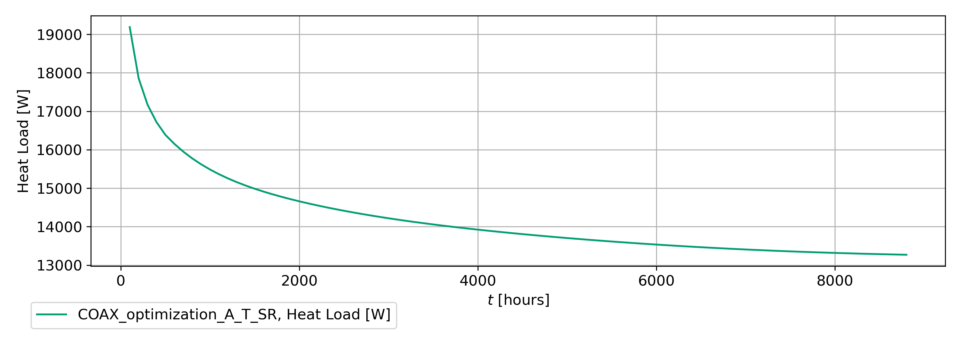
Fig. 3: Power yield during a year of constant operation of the coaxial BHE with an optimized flow rate and pipe insulation design.
The COP of the fluid circulation pump during the simulated period is shown in Fig. 4. The last value of this time-variable COP is used to test the COP constraint in the optimization process (see Theory section).
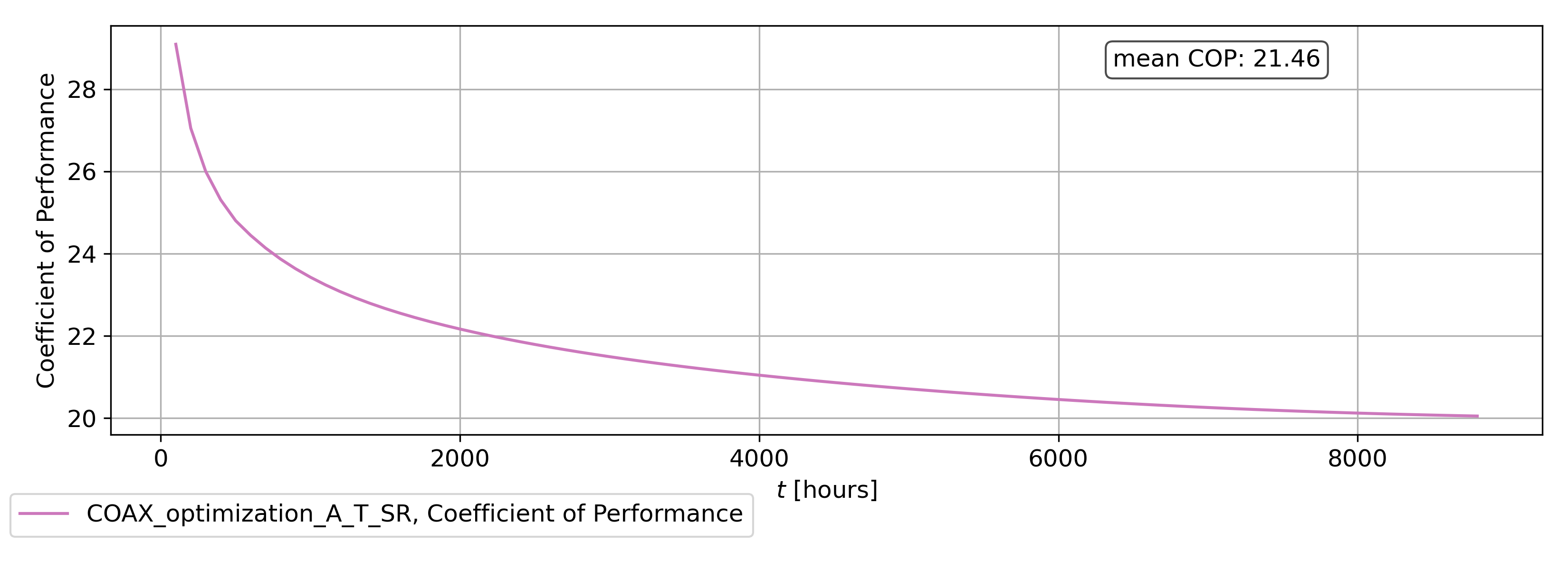
Fig. 4: COP of the fluid circulation pump during a year of constant operation of the coaxial BHE with an optimized flow rate and pipe insulation design.
Optimal flow rate and radius of the inner pipe
In the second simulation, the radius of the inner pipe in the coaxial BHE is optimized for the maximum power yield, for which the result is shown in Fig. 5. The inner pipe has a radius of 36 mm.
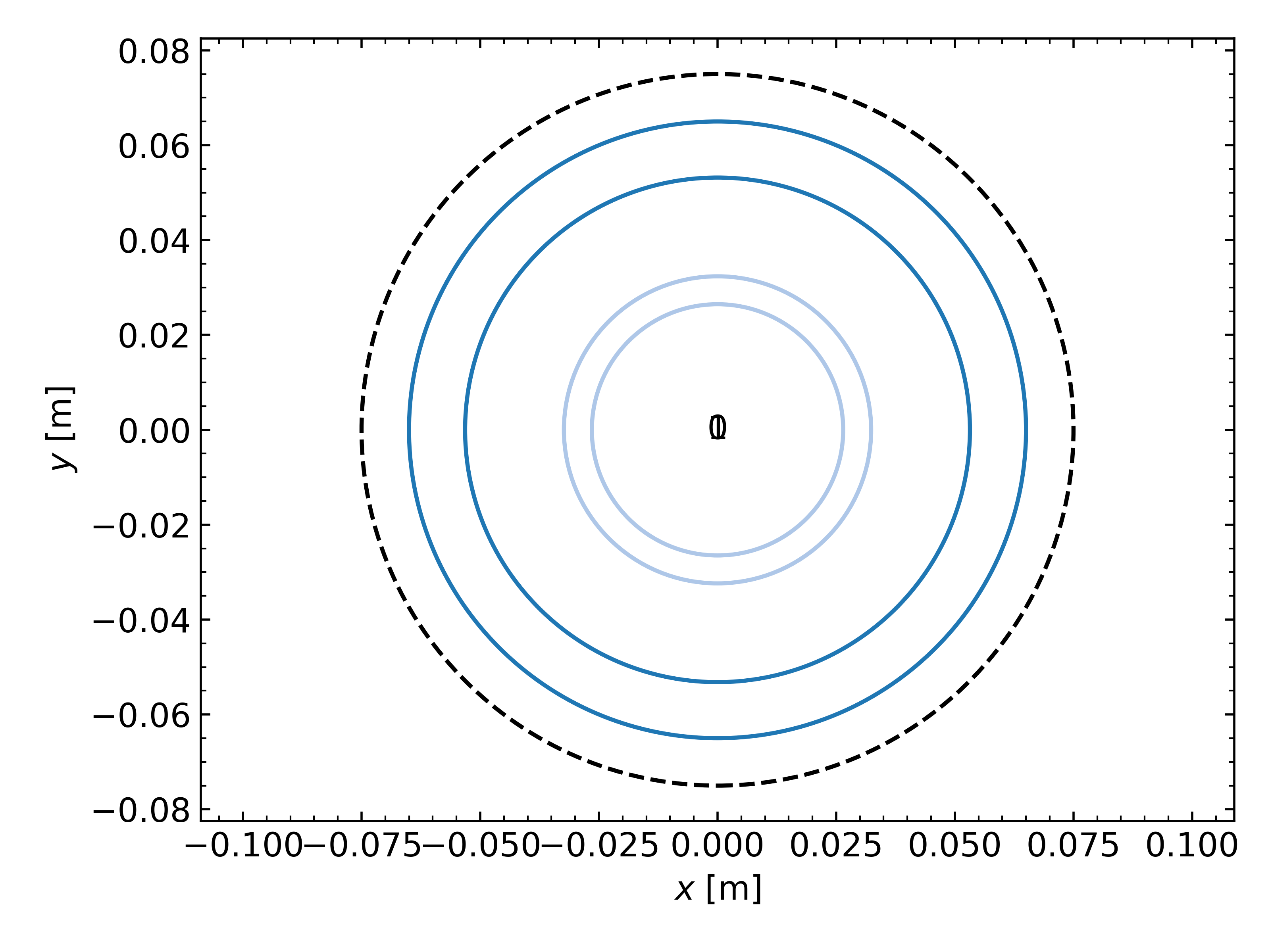
Fig. 5: Cross-section of the BHE design in the second optimization simulation for maximum power yield of the system.
Here, the flow rate and the radius of the inner pipe are optimized under the condition of a minimum COP of the circulation pump of 20 and an imposed pumping pressure of 1.7 bar.
The lack of insulation in the outlet is clearly reflected by the heat loss in the working fluid during upward transport in the inner pipe of the BHE (see Fig. 6).
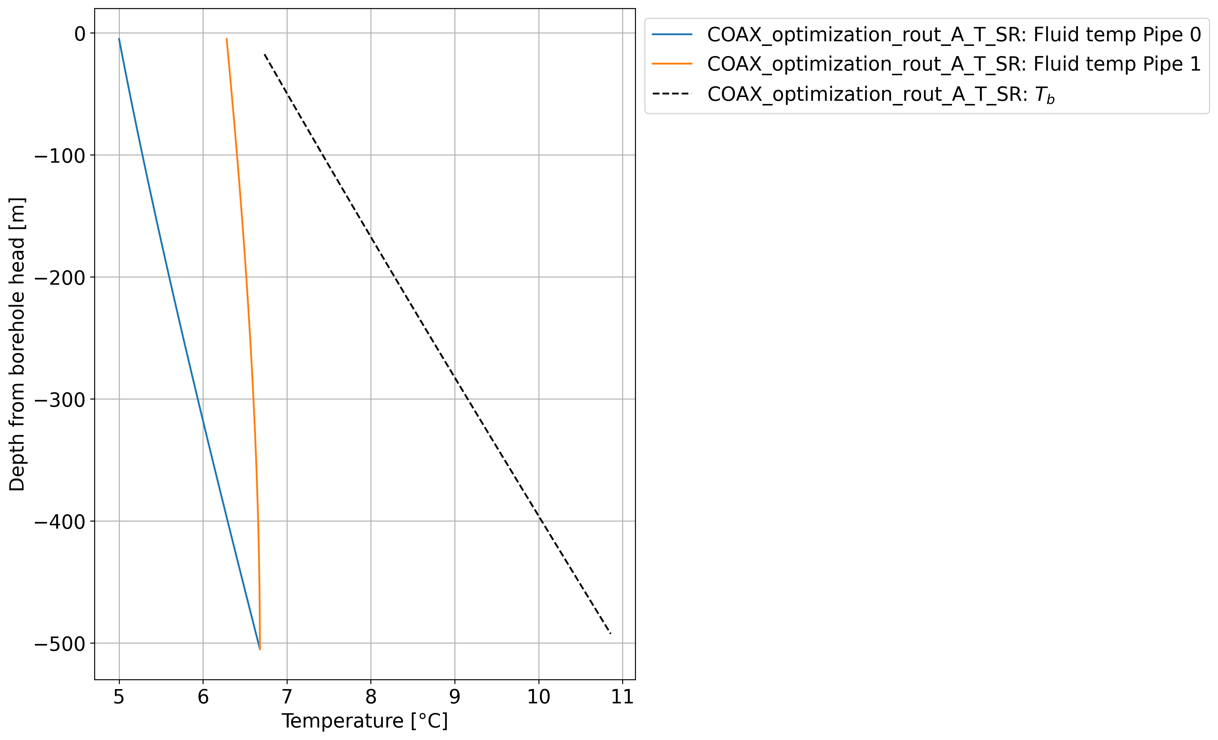
Fig. 6: Fluid and borehole wall temperatures after half a year of operation of the coaxial BHE with an optimized flow rate and radius of the inner pipe.
The power yield that follows from the simulation is shown in Fig. 7.
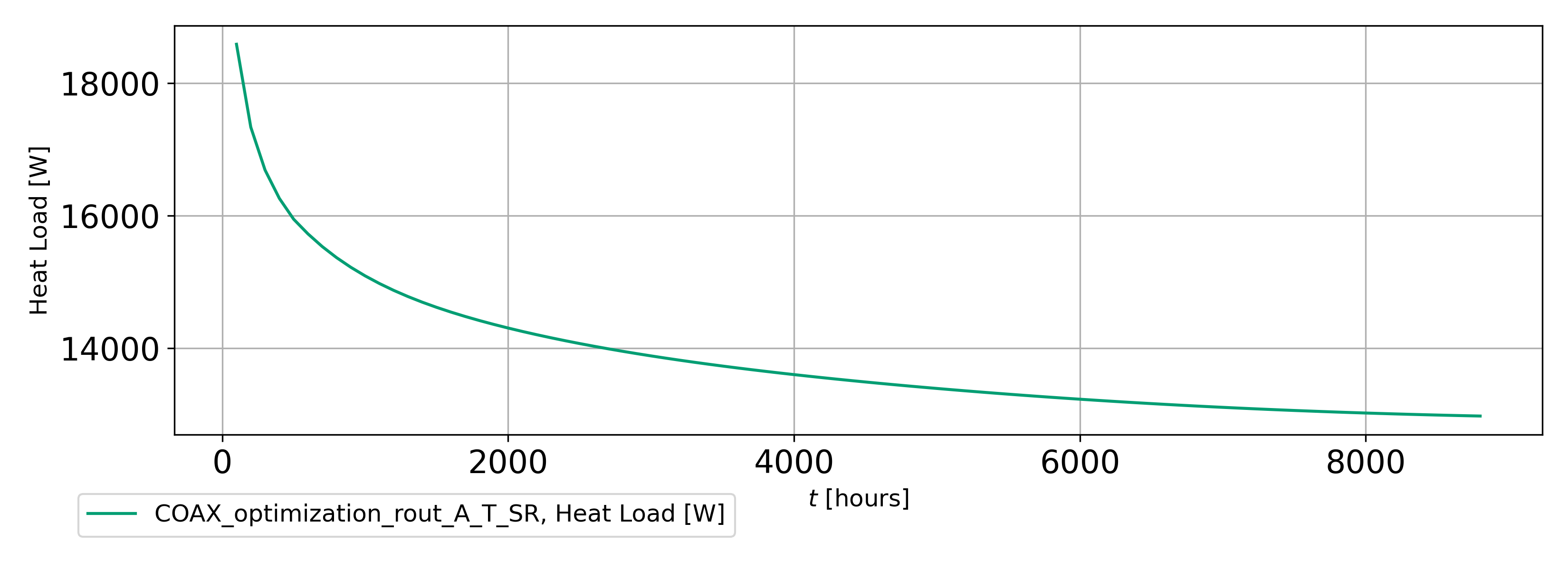
Fig. 7: Power yield during a year of operation of the coaxial BHE with an optimized flow rate and radius of the inner pipe.